First Order Ordinary Differential Equations
Existence and Uniqueness
Definition. Given an open interval $I$ that contains $t_0$, a solution of the initial value problem
\[{\mathrm{d}x \over \mathrm{d}t} = f(x, t) \quad \text{with} \quad x(t_0) = x_0\]on $I$ is a differentiable function $x(t)$ defined on $I$, with $x(t_0) = x_0$ and $x’(t) = f(x, t)$ for all $t \in I$.
The main point is that we allow a solution to be defined only for some interval instead of every value in $\mathbb{R}$.
Theorem. If $f(x, t)$ and $\partial f / \partial x$ are continuous for $a < x < b$ and $c < t < d$, then for any $x_0 \in (a, b)$ and $t_0 \in (c, d)$ the initial value problem has a unique solution on some open interval $I$ containing $t_0$.
The freedom to specify the interval on which the solution of an equation exists is necessary.
Example. The initial value problem
\[{\mathrm{d}x \over \mathrm{d}t} = x^2 \quad \text{with} \quad x(0) = x_0\]has the solution
\[x(t) = {1 \over x_0^{-1} - t}\]The solution tends to zero as $t \to \infty$. When $x_0 > 0$, by the time $t = t_0^{-1}$, the solution “blows up” and become infinite. Therefore, we can define the solution only on the interval $(-\infty, x_0^{-1})$ and it is called the maximal interval of existence.
Trivial Equations
Proposition. Consider a differential equation of the form
\[{\mathrm{d} y \over \mathrm{d} x} = f(x)\]By the Fundamental Theorem of Calculus, the general solution is anti-derivative $F$ of $f$, i.e.
\[y(x) = F(x) + c\]where $c$ is determined by an initial condition.
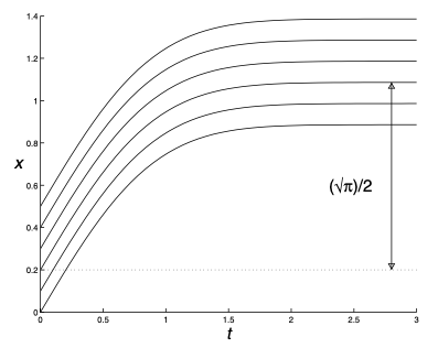
Sometimes we might not be able to write down an explicit form for the solution, but it can still be possible to describe qualitatively the behaviour of it. For example, for the equation
\[{\mathrm{d} x \over \mathrm{d} t} = e^{-t^2}\]the general solution is the Gaussian Integral
\[x(t) = x_0 + \int_0^t e^{-\tilde{t}^2} \mathrm{d} \tilde{t}\]in which there is no explicit form for the anti-derivative of $e^{-t^2}$. However, we have
\[\int_0^\infty e^{-t^2} \mathrm{d}t = {\sqrt{\pi} \over 2}\]So, we can say, since $x’(t) > 0$ for all $t$, $x(t)$ increases as $t$ increases and $x(t) \to x_0 + \sqrt{\pi}/2$.
Autonomous Equations
Definition. A differential equation is autonomous if it doesn’t explicitly depend on the independent variable, i.e.
\[{\mathrm{d} x \over \mathrm{d} t} = f(x)\]
An explict solution might be able to be found by methods below such as by separating the variables, but we can also try to understand the solutions “qualitatively”.
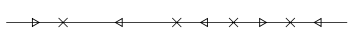
Definition. The phase diagram is a diagram that shows the qualitative behaviour of an autonomous equation by identifying the equilibria and their stability. The points with rate of change equals zero, i.e. $f(x^\ast) = 0$, are the equilibria. In between there are arrows, in which up/right arrow represents the solution is increasing, i.e. $f(x) > 0$, and down/left arrow represents the solution is decreasing, i.e. $f(x) < 0$.
For example,
Definition. An equilibrium is stable if it is attacting nearby solutions. More precisely, given any $\epsilon > 0$, there exists a $\delta > 0$ such that
\[|x_0 - x^\ast| < \delta \quad \implies \quad |x(t) - x^\ast| < \epsilon, \forall t \ge 0\]An equilibrium is unstable if it is not stable, i.e. it repels nearby solutions. It means there exists an $\epsilon > 0$ such that for any $\delta > 0$, $\vert x_0 - x^\ast \vert < \delta$ but $\vert x(t) - x^\ast \vert > \epsilon$ for some $t > 0$.
For example, the equilibria above are labeled with the corresponding stability:
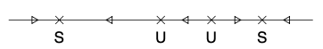
Proposition. The stability of equilibria is determined by the following conditions:
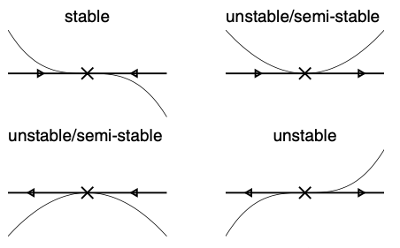
Definition. The differential equation has a bifurcation near an equilibrium $x^\ast$ if a small change to $f$ will change the phase diagram drastically. Otherwise, it is structurally stable.
For example, for the top right case in the diagram above, increasing $f(x)$ by any constant $c > 0$ will make the equilibrium gone.
An example of its application can be found in Practical Examples.
Separable Equations
Proposition. Consider a differential equation of the form
\[{\mathrm{d}x \over \mathrm{d}t} = f(x)g(t)\]and assume $f(x)$ is sufficiently smooth so that it has a unique solution for any specified initial condition.
If $f(x(s)) = 0$ for some $s$, it implies $x(t) = x(s)$ for all $t \in \mathbb{R}$, i.e. a constant function. We can see that if $x(t) = x(s)$, $x’(t) = 0$, which satisfies the differential equation and therefore it is really the unique solution to that. It implies that either $f(x(t)) = 0$ for all $t \in \mathbb{R}$ or $f(x(t)) \not = 0$ for all $t \in \mathbb{R}$.
If $f(x(t)) \not= 0$ for all $t \in \mathbb{R}$, we can divide both sides of the equation by $f(x)$, i.e.
\[{1 \over f(x)} {\mathrm{d}x \over \mathrm{d}t} = g(t)\]Let $H(x)$ be the anti-derivative of $1/f(x)$, by chain rule, we have
\[{\mathrm{d} \over \mathrm{d}t} H(x(t)) = H'(x) {\mathrm{d}x \over \mathrm{d}t} = {1 \over f(x)} {\mathrm{d}x \over \mathrm{d}t} = g(t)\]By integrating both sides we have
\[H(x(t)) = \int g(t) \mathrm{d}t\]Let $G(t)$ be the anti-derivative of $g(t)$, we have $H(x(t)) = G(t) + c$, and by substituting the initlal condition $x(t_0) = x_0)$ into the equation,
\[H(x_0) = G(t_0) + c \implies c = H(x_0) - G(t_0) \implies H((x(t)) - H(x_0) = G(t) - G(t_0)\]Hence, by Fundamental Theorem of Calculus, the solution is
\[\int_{x_0}^{x(t)} {1 \over f(x)} \mathrm{d}x = \int_{t_0}^{t} g(\tilde{t}) \mathrm{d}\tilde{t}\]
This method frequently gives solution with absolute sign as
\[\int_{x_0}^{x(t)} {1 \over f(x)} \mathrm{d}(f(x)) = \ln |f(x(t))| - \ln |f(x_0)|\]Most of the time, the absolute sign can be eliminated by renaming the variables with a different condition.
Example. For equation $y’ = xy$, note that $y = 0$ is a solution.
Assume $y \not= 0$ for all $x$, we have
\[\begin{align*} \int {1 \over y } \mathrm{d}y &= \int x \mathrm{d}x \\ \ln |y| &= {x^2 \over 2} + c \\ |y| &= Ae^{x^2/2} \quad \text{where } A = e^c > 0 \\ y &= Be^{x^2/2} \quad \text{where } B \in \mathbb{R} \end{align*}\]We can see that the general solution includes the particular solution $y = 0$.
Linear Equations by Integrating Factors
Proposition. For a general linear differential equation
\[x'(t) + p(t)x(t) = q(t)\]By multiplying both sides by $I(t)$, we have
\[I(t)x'(t) + I(t)p(t)x(t) = I(t)q(t)\]Consider the derivative of $I(t)x(t)$, by product rule,
\[{\mathrm{d} \over \mathrm{d}t}I(t)x(t) = I(t)x'(t) + I'(t)x(t)\]Thus, in order for the L.H.S. to be grouped together, we need to have
\[I(t)p(t) = I'(t)\]which is a separable equation. Therefore,
\[\int {1 \over I} \mathrm{d}I = \int p(t) \mathrm{d}t\]and we have the integrating factor
\[I(t) = \exp({\int p(t) \mathrm{d}t})\]Substituting it back to the linear differential equation,
\[\begin{align*} x'(t)I(t) + p(t)x(t)I(t) &= q(t)I(t) \\ {\mathrm{d} \over \mathrm{d}t} I(t)x(t) &= q(t)I(t) \\ I(t)x(t) &= \int q(t)I(t) \mathrm{d}t \\ x(t) &= {1 \over I(t)} \int q(t)I(t) \mathrm{d}t \end{align*}\]which is the general solution.
Exact Equations
Proposition. Consider a differential equation of the form
\[f(x, y) + g(x, y){\mathrm{d}y \over \mathrm{d}x} = 0\]Suppose that $x$ and $y$ are related implicitly by $F(x, y) = c$, by chain rule,
\[{\mathbf{d}F \over \mathrm{d}x} = {\partial F \over \partial x} {\mathrm{d}x \over \mathrm{d}x} + {\partial F \over \partial y} {\mathrm{d}y \over \mathrm{d}x} = 0\]Comparing that to the differential equation, we have
\[{\partial F \over \partial x} = f(x, y) \quad \text{and} \quad {\partial F \over \partial y} = g(x, y)\]Since the order of taking two partial derivatives does not matter, we have
\[{\partial f \over \partial y} = {\partial g \over \partial x}\]as the necessary and sufficient condition for the differential equation to be “exact”.
We then have
\[F(x, y) = \int f(x, y) dx + C(y) \quad \text{and} \quad {\partial F \over \partial y} = {\partial \over \partial y} \int f(x, y) dx + {\mathrm{d} C \over \mathrm{d} y} = g(x, y)\]and the solution to the equation is
\[F(x, y) = C\]
It is possible to turn an equation into an exact equation if it is multiplied by the correct integrating factors. Consider the equation
\[f(x, y) + g(x, y) {\mathrm{d}y \over \mathrm{d}x} = 0\]Multiplying both sides by $I(x, y)$ we have
\[f(x, y)I(x, y) + g(x, y) I(x, y) {\mathrm{d}y \over \mathrm{d}x} = 0\]Thus, in order for the equation to have be exact, we have
\[\begin{align*} {\partial \over \partial y} f(x, y) I(x, y) &= {\partial \over \partial x} g(x, y) I(x, y) \\ I {\partial f \over \partial y} + f {\partial I \over \partial y} &= I {\partial g \over \partial x} + g {\partial I \over \partial x} \\ \left( {\partial f \over \partial y} - {\partial g \over \partial x} \right) I &= g {\partial I \over \partial x} - f {\partial I \over \partial y} \end{align*}\]which is a PDE which is no easier to solve.
However, if $I$ is a function consists only of $x$, then
\[\left( {\partial f \over \partial y} - {\partial g \over \partial x} \right) I = g {\mathrm{d} I \over \mathrm{d} x}\]If
\[{1 \over g} \left( {\partial f \over \partial y} - {\partial g \over \partial x} \right)\]depends only on $x$, it becomes a seprable equation and we can solve for $I(x)$.
Homogeneous Equations
Definition. A first order differential equation is said to be homogeneous if it can be written in the form
\[{\mathrm{d} y \over \mathrm{d} x} = F({y \over x})\]
Proposition. For a homogeneous differential equation, by substituting $u = y/x$, we have $y = ux$ and by product rule,
\[{\mathrm{d} y \over \mathrm{d} x} = u + x {\mathrm{u} u \over \mathrm{d} x}\]Hence,
\[x {\mathrm{d} u \over \mathrm{d} x} = F(u) - u\]is a separable equation.
Bernoulli Equations
Proposition. Consider a differential equation of the form
\[{\mathrm{d}y \over \mathrm{d} x} + p(x)y = q(x)y^n\]If $n = 0, 1$, it is a linear equation and can be solved by finding the integrating factors.
If $n \ge 2$, let $u = y^{1-n}$,
\[u' = (1 - n) y^{-n} y'\]Hence, by multiplying $(1 - n) y^{-n}$ to the original differential equation, we have
\[\begin{align*} (1 - n) y^{-n} y' + (1 - n) p(x) y^{1-n} &= (1 - n)q(x) \\ u' + (1 - n) p(x) u &= (1 - n)q(x) \end{align*}\]which becomes a linear differential equation and can be solved by integrating factors.
References
- James C. Robinson An Introduction to Ordinary Differential Equations, 2004 - Chapter 5 - 10
- https://youtu.be/u0vbm1T420g