Second Order Ordinary Differential Equations
Existence and Uniqueness
Theorem. Given a function $f(x_2, x_1, t)$. Suppose that $f$, $\partial f / \partial x_1$ and $\partial f / \partial x_2$ are continuous functions for $a_1 < x_1 < a_2$, $b_1 < x_2 < b_2$ and $t_1 < t < t_2$. Then for all initial conditions
\[x(t_0) = x_0 \quad \text{and} \quad x'(t_0) = y_0\]with $a_1 < x_0 < x_2$, $b_1 < y_0 < b_2$ and $t_1 < t_0 < t_2$ there exists a unique solution of
\[x'' = f(x', x, t)\]on some interval $I$ containing $t_0$, i.e. a continuous function with two continuous derivatives satisfying the the initial conditions and the differential equation on $I$.
Linearity
Proposition. The differential operator $L$ defined by
\[L[x](t) = {\mathrm{d}^2x \over \mathrm{d}t^2}(t) + p(t) {\mathrm{d}x \over \mathrm{d}t}(t) + q(t)x(t)\]is linear.
Proof.
Consider a homogeneous second order linear differential equation
\[{\mathrm{d}^2x \over \mathrm{d}t^2} + p(t) {\mathrm{d}x \over \mathrm{d}t} + q(t) x = 0\]which is equivalent to
\[L[x] = 0\]Suppose $x_1$ and $x_2$ are two solutions to the equation, for all $\alpha, \beta \in \mathbb{R}$, we have
\[\begin{align*} L[\alpha x_1 + \beta x_2] &= {\mathrm{d}^2 \over \mathrm{d}t^2}(\alpha x_1 + \beta x_2) + p(t) {\mathrm{d} \over \mathrm{d}t}(\alpha x_1 + \beta x_2) + q(t) (\alpha x_1 + \beta x_2) \\ &= \alpha \left[ {\mathrm{d}^2 x_1 \over \mathrm{d}t^2} + p(t) {\mathrm{d} x_1 \over \mathrm{d}t} + q(t) x_1) \right] + \beta \left[ {\mathrm{d}^2 x_2 \over \mathrm{d}t^2} + p(t) {\mathrm{d} x_2 \over \mathrm{d}t} + q(t) x_2) \right] \\ &= \alpha L[x_1] + \beta L[x_2] = 0 \end{align*}\]so $\alpha x_1 + \beta x_2$ is also a solution. Hence, $L$ is linear.
Linear Independence of Functions
Definition. The functions $x_1(t), …, x_n(t)$ are linearly independent on an interval $I$ if
\[a_1x_1(t) + \cdots + a_nx_n(t) = 0 \quad \implies \quad a_1 = \cdots = a_n = 0\]
Proposition. Two linearly independent solutions are necessary and sufficient to obtain all possible solutions of homogeneous second order ODE.
Proof.
Given a homogeneous second order ODE. Suppose $x_1(t)$ is the solution satisfying
\[x_1(t_0) = 1 \quad \text{and} \quad x_1'(t_0) = 0\]and $x_2(t)$ is the solution satisfying
\[x_2(t_0) = 0 \quad \text{and} \quad x_1'(t_0) = 1\]By the existence and uniqueness theorem, both should exist but one cannot be a multiple of the other. Hence, at least two linearly independent solutions are necessary.
Given two solutions that are linearly independent like above and for any given initial condition
\[x(t_0) = x_0 \quad \text{and} \quad x'(t_0) = x_0'\]We have the following system of linear equations
\[\begin{pmatrix} x_1(t_0) & x_2(t_0) \\ x_1'(t_0) & x_2'(t_0) \\ \end{pmatrix} \begin{pmatrix} \alpha \\ \beta \end{pmatrix} = \begin{pmatrix} x_0 \\ x_0' \end{pmatrix}\]As the two solutions are linearly independent, the system has a unique solution. Hence, two linearly independent solutions are sufficient to form any solution.
The Wronskian
Definition. The Wronskian of two functions $x_1(t)$ and $x_2(t)$ is defined by
\[W[x_1, x_2](t) = \begin{vmatrix} x_1(t) & x_2(t) \\ x_1'(t) & x_2'(t) \end{vmatrix} = x_1(t)x_2'(t) - x_2(t)x_1'(t)\]
Proposition. The function $x_1$ and $x_2$ are linearly independent on an interval $I$ iff their Wronskian $W[x_1, x_2](t) \not \equiv 0$ on $I$. Hence, if $W[x_1, x_2](t) = 0$ for any $t \in I$, then $x_1$ and $x_2$ are linearly dependent.
Proof.
Given a homogeneous second order differential equation
\[{\mathrm{d}x \over \mathrm{d}t^2} + p(t) {\mathrm{d}x \over \mathrm{d}t} + q(t)x = 0\]with two solutions $x_1$ and $x_2$. Then
\[W(t) = x_1(t)x_2'(t) - x_2(t)x_1'(t) \quad \text{and} \quad W'(t) = x_1(t)x_2''(t) - x_1''(t)x_2(t)\]and we have
\[\begin{align*} W'(t) + p(t)W(t) &= x_1(t) [x_2''(t) + p(t)x_2'(t)] - x_2(t) [x_1''(t) + p(t)x_1'(t)] \\ &= x_1(t)[-q(t)x_2(t)] - x_2(t)[-q(t)x_1(t)] \\ &= 0 \end{align*}\]Therefore, we have the Wronskian satisfying the differential equation
\[W'(t) = -p(t)W(t)\]If $W(t) = 0$, $W’(t) = 0$, then $W(t) \equiv 0$ for all $t \in I$.
If $W(t) \not = 0$, $\vert W(t) \vert = e^{\int -p(t) \mathrm{d}t}$, then $W(t) \not = 0$ for all $t \in I$.
Homogeneous + Linear + Constant Coefficient
Proposition. Consider a differential equation of the form
\[ax'' + bx' + c = 0\]Let $x(t) = e^{kt}$ be the solution. Then
\[(ak^2 + bk + c) e^{kt} = 0\]Since $e^{kt}$ is non-zero, we can divide both side with that and end up with a quadratic equation
\[ak^2 + bk + c = 0\]which is called the auxiliary/characteristic equation.
Proposition. If the characteristic equation has two distinct real roots $k_1$ and $k_2$, then the general solution is
\[x(t) = Ae^{k_1 t} + Be^{k_2 t}\]
Proposition. If the characteristic equation has one repeated root $k$, then the general solution is
\[x(t) = (A + Bt)e^{kt}\]
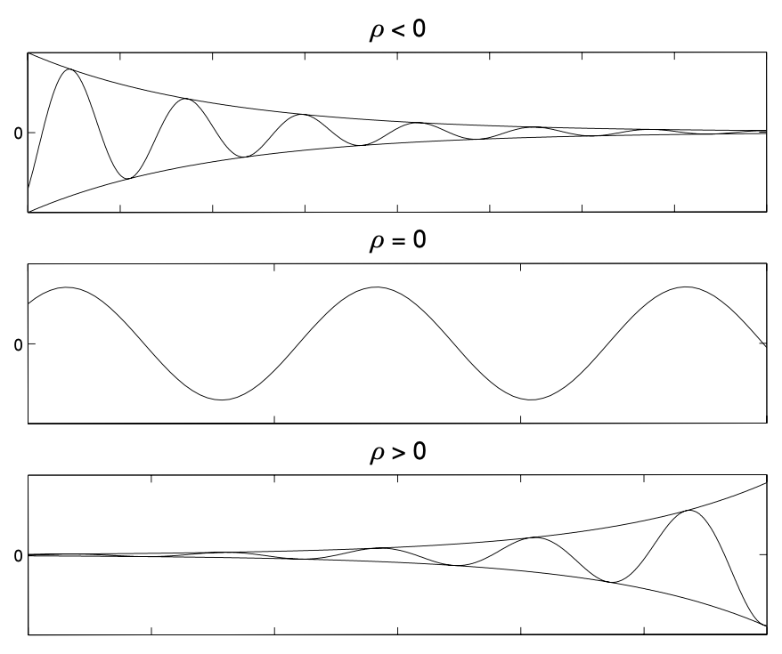
Proposition. If the characteristic equation has two complex roots $k = \rho \pm \omega i$, then the general solution is
\[x(t) = e^{\rho t}(A \cos \omega t + B \sin \omega t)\]Proof.
The complex roots can be handled just like they are real, i.e.
\[x(t) = Ce^{(\rho + \omega i)t} + De^{(\rho - \omega i)t}\]We want to restrict the solutions to be real. As $e^{(\rho - \omega i)t}$ is the complex conjugate of $e^{(\rho + \omega i)t}$, by having $D$ being complex comjungate of $C$, we will restrict the right hand side to be real as well.
Therefore, let $C = \alpha + \beta i$,
\[\begin{align*} x(t) &= 2 \text{Re}[Ce^{(\rho + \omega i)t}] \\ &= 2e^{\rho t} \text{Re}[(\alpha + \beta i)(\cos \omega t + i \sin \omega t)] \\ &= 2e^{\rho t} (\alpha \cos \omega t - \beta \sin \omega t) \\ &= e^{\rho t} (A \cos \omega t + B \sin \omega t) \end{align*}\]
We can further combine $A \cos \omega t + B \sin \omega t$ to one oscillating term $M \cos (\omega t - \theta)$, the amplitude is controlled by the sign of $\rho$. If $\rho < 0$, the solution decays to $0$. If $\rho = 0$, we have pure oscillations. If $\rho > 0$, the solution grows exponentially fast.
Inhomogeneous + Linear + Constant Coefficients
Proposition. Consider a differential equation of the form
\[L[x] = ax'' + bx' + cx = f(t)\]Let $x_1$ and $x_2$ be two linearly independent solutions for the equation $L[x] = 0$ and $x_p$ be a particular solution of $L[x] = f(t)$. Then the general solution for the differential equation is
\[x(t) = Ax_1(t) + Bx_2(t) + x_p(t)\]
Definition. $x_h(t) = Ax_1(t) + Bx_2(t)$ is called the complimentary function and $x_p(t)$ is called the particular integral.
Finding $x_p$ involves some educated guess. Common choices are
| $f(t)$ | $x_p(t)$ |
| $t^n$ | $c_nt^n + \cdots + c_0$ |
| $ce^{kt}$ | $Ce^{kt}$ |
| $\alpha \sin \sigma t + \beta \cos \sigma t$ | $C \sin \sigma t + D \sin \sigma t$ |
In case $x_p(t)$ is one of the solution in $x_h(t)$, we can multiply it by $t$ or $t^2$ to form a new particular integral.
If $f(t) = \alpha f_1(t) + \beta f_2(t)$, then $x_p = \alpha x_{p1} + \beta x_{p2}$.
If $f(t) = f_1(t)f_2(t)$, then $x_p = x_{p1}x_{p2}$. For example, the particular integral for $f(t) = te^{-t}\cos 2t$ is
\[x_p(t) = (At + B)e^{-t}\cos 2t + (Ct + D)e^{-t}\sin 2t\]Reduction of Order
This is the technique for finding the second linearly independent solution in case we already know one.
Proposition. For the case of having coefficients as functions of $t$, i.e.
\[a(t){\mathrm{d}^2 x \over \mathrm{d}t^2} + b(t){\mathrm{d}x \over \mathrm{d}t} + c(t)x = 0\]If we happen to know one solution $u(t)$ of the equation, let $x(t) = u(t)y(t)$, we have
\[x' = u'y + uy' \quad \text{and} \quad x'' = u''y + 2u'y' + uy''\]Substituting it back and grouping the terms containing $y$, we have
\[\begin{align*} y[a(t)u'' + b(t)u' + c(t)u] + y'[2a(t)u' + b(t)u] + y''[a(t)u] &= 0 \\ y'[2a(t)u' + b(t)u] + y''[a(t)u] &= 0 \end{align*}\]Thus, by putting $z = y’$
\[[a(t)u(t)]z' + [2a(t)u'(t) + b(t)u(t)]z = 0\]which is a first order differential equation that can be solved by the method of integrating factors.
Variation of Parameters
This is the technique for finding the particular integral in case we already know two linear independent solutions of the homogeneous equation.
Proposition. Consider a differential equation
\[{\mathrm{d}^2 x \over \mathrm{d}t^2} + p(t){\mathrm{d}x \over \mathrm{d}t} + q(t)x = f(t)\]If we know two linearly independent solutions $x_1(t)$ and $x_2(t)$ for the homogeneous problem, let
\[x_p(t) = u_1(t)x_1(t) + u_2(t)x_2(t)\]which is like by changing the constants $A$ and $B$ of the general solution to unknown functions $u_1(t)$ and $u_2(t)$. Then
\[x_p'(t) = u_1'(t)x_1(t) + u_1(t)x_1'(t) + u_2'(t)x_2(t) + u_2(t)x_2'(t)\]In order to keep the second derivative manageable, we impose the condition that
\[u_1'x_1 + u_2'x_2 = 0\]Thus,
\[x_p''(t) = u_1(t)x_1''(t) + u_1'(t)x_1'(t) + u_2'(t)x_2'(t) + u_2(t)x_2''(t)\]Substituting them back to the original equation to get
\[u_1[x_1'' + p(t)x_1' + q(t)x_1] + u_2[x_2'' + p(t)x_2' + q(t)x_2] + u_1'x_1' + u_2'x_2' = f(t)\]As $x_1$ and $x_2$ are the solutions of the homogeneous equation, we have
\[u_1'x_1' + u_2'x_2' = 0\]Therefore, we have the following system of equations
\[\begin{cases} u_1'x_1 + u_2'x_2 = 0 \\ u_1'x_1' + u_2'x_2' = f(t) \end{cases} \implies \begin{pmatrix} x_1 & x_2 \\ x_1' & x_2' \end{pmatrix} \begin{pmatrix} u_1' \\ u_2' \end{pmatrix} = \begin{pmatrix} 0 \\ f(t) \end{pmatrix}\]The array on the L.H.S is the Wronskian of $x_1$ and $x_2$ and is non-zero for linearly independent solutions.
Hence,
\[\begin{pmatrix} u_1' \\ u_2' \end{pmatrix} = {1 \over W(t)} \begin{pmatrix} x_2' & -x_2 \\ -x_1' & x_1 \end{pmatrix} \begin{pmatrix} 0 \\ f(t) \end{pmatrix}\]and the required particular integral is
\[x_p(t) = -x_1(t) \int {x_2(t)f(t) \over W(t)} \mathrm{d}t + x_2(t) \int {x_1(t)f(t) \over W(t)} \mathrm{d}t\]
References
- James C. Robinson An Introduction to Ordinary Differential Equations, 2004 - Chapter 11, 12, 14, 17, 18