Series Solutions
Even though we can solve differential equations by methods mentioned previously, it is still useful to find solution in terms of power series for computational purpose.
Definition. A function $f$ is analytic at a point $x = x_0$ if it has a Taylor series expansion about $x = x_0$, i.e.
\[f(x) = \sum_{n=0}^\infty {f^{(n)}(x_0) \over n!} (x - x_0)^n\]with a raidus of convergence $\rho > 0$.
Definition. An orderinary point $x_0$ of a differential equation
\[P(x) y'' + Q(x) y' + R(x) y = 0\]is a point such that $p = Q/P$ and $q = R/P$ are analytic at $x_0$.
Definition. A singular point of a differential equation is a point that is not ordinary, i.e. $P(x_0) = 0$ and at least one of $Q$ and $R$ is not zero at $x_0$.
Ordinary Points
Theorem. If $x_0$ is an ordinary point of the differential equation
\[P(x) y'' + Q(x) y' + R(x) y = 0\]then the general solution is of the form
\[y = \sum_{n=0}^\infty a_n (x - x_0)^n = a_0 y_1(x) + a_1 y_2(x)\]where $a_0$ and $a_1$ are arbitrary and
$y_1$ and $y_2$ are two power series solutions that are analytic at $x_0$,
$y_1$ and $y_2$ form a fundamental set of solutions,
the radius of convergence for each of the series solutions is at least as large as the minimum of the radii of convergence of the series for $p = Q/P$ and $q = R/P$.
Example. For the differential equation
\[y'' + y = 0\]Consider a power series about $x_0 = 0$ that converges in some interval $\vert x \vert < \rho$, we have
\[y = \sum_{n=0}^\infty a_n x^n \quad \text{and} \quad y' = \sum_{n=1}^\infty n a_n x^{n-1} \quad \text{and} \quad y'' = \sum_{n=2}^\infty n(n-1) a_n x^{n-2}\]Then
\[\begin{align*} \sum_{n=2}^\infty n(n-1) a_n x^{n-2} + \sum_{n=0}^\infty a_n x^n &= 0 \\ \sum_{n=0}^\infty (n+2)(n+1) a_{n+2} x^n + \sum_{n=0}^\infty a_n x^n &= 0 \\ \end{align*}\]For this equation to be satisfied for all $x$, we need to have
\[(n+2)(n+1) a_{n+2} + a_n = 0\]For the even-numbered coefficients
\[a_2 = - {a_0 \over 2!} \quad \text{and} \quad a_4 = - {a_2 \over 3 \cdot 4} = {a_0 \over 4!} \quad \text{and} \quad a_{2k} = {(-1)^k \over (2k)!} a_0\]For the odd-numbered coefficients
\[a_3 = - {a_1 \over 3!} \quad \text{and} \quad a_5 = - {a_3 \over 4 \cdot 5} = {a_1 \over 5!} \quad \text{and} \quad a_{2k+1} = {(-1)^k \over (2k + 1)!} a_1\]Hence,
\[y = a_0 \sum_{n=0}^\infty {(-1)^n \over (2n)!} x^{2n} + a_1 \sum_{n=0}^\infty {(-1)^n \over (2n + 1)!} x^{2n + 1}\]Be noted that the series solutions provide only a local approximation about $x = 0$ if they are truncated.
Base on the above theorem, as $P(x) = 1, Q(x) = 0, R(x) = 1$ and $x_0 = 0$ is an ordinary point, we can conclude that
-
the solutions converge for all $x$,
-
the two solutions are linearly independent and form a fundamental set of solutions.
We can confirm their convergence by ratio test and found that they really converge for all $x$. On the other hand, let
\[C(x) = \sum_{n=0}^\infty {(-1)^n \over (2n)!} x^{2n} \quad \text{and} \quad S(x) = \sum_{n=0}^\infty {(-1)^n \over (2n + 1)!} x^{2n + 1}\]We found that
\[C'(x) = -S(x) \quad \text{and} \quad S'(x) = C(x)\]Their Wronskian at $x = 0$ is
\[W[C, S](0) = \begin{vmatrix} C(0) & S(0) \\ -S(0) & C(0) \end{vmatrix} = \begin{vmatrix} 1 & 0 \\ 0 & 1 \end{vmatrix} = 1\]and therefore the two solutions are indeed linearly independent.
According to the list of Power Series, the two series solutions are indeed $\sin x$ and $\cos x$, which matches the solutions we found by other techniques. The function $\sin x$ can in fact be defined as the unique solution of the IVP $y’’ + y = 0, y(0) = 0, y’(0) = 1$. Similarily, the function $\cos x$ can be defined as the unique solution of the IVP $y’’ + y = 0, y(0) = 1, y’(0) = 0$
For ratio test to work, we have to find an explicit formula for the coefficients, and sometimes it will be hard or even not feasible. The theorem provides a good way to find a lower bound of radius of convergence without even solving the equation.
Example. For the Legendre equation
\[(1 - x^2)y'' - 2xy' + \alpha(\alpha + 1)y = 0\]As $P(x) = 1 - x^2$, $Q(x) = -2x$ and $R(x) = \alpha(\alpha + 1)$ are polynomials, the distance of $x = 0$ from zeros of $P(x)$ is the radius of convergence, i.e. $P(x) = 0 \implies x = \pm 1$ so $\rho = 1$ or $\vert x \vert < 1$ for series solutions about $x = 0$.
Cauchy-Euler Equations
Definition. The Cauchy-Euler equations or equidimensional equations are the differential equations of the form
\[L[y] = x^2 y'' + ax y' + by = 0\]where $a, b$ are real constants.
Proposition. Assume a solution is of the form $y(x) = x^r$ for $x > 0$. Then
\[L[x^r] = x^r[r(r-1) + ar + b] = 0\]Cancelling the $x^r$ factor and we obtain the indicial equation
\[F(r) = ar(r-1) + br + c = 0\]and the roots are
\[r_1, r_2 = {-(a - 1) \pm \sqrt{(a - 1)^2 - 4b} \over 2}\]
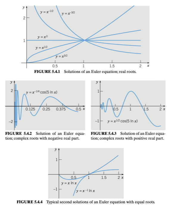
Proposition. If the indicial equation has two real roots $r_1$ and $r_2$, then the general solution is
\[y(x) = Ax^{r_1} + Bx^{r_2}\]
Proposition. If the indicial equation has one repeated root $r$, then the general solution is
\[y(x) = Ax^{r} + Bx^{r}\ln x = (A + B\ln x)x^r\]Proof.
The other solution can be derived by reduction of order.
Alternatively, note that $F(r) = (r - r_1)^2$ which implies $F’(r_1) = 0$ as well.
By differentiating the differential equation with respect to $r$, we have
\[{\partial \over \partial r} L[x^r] = {\partial \over \partial r} x^r F(r)\]and therefore
\[L[x^r \ln x] = (r - r_1)^2 x^r \ln x + 2(r - r_1) x^r\]in which the R.H.S. is zero for $r = r_1$. Hence, $x^{r_1} \ln x$ is the second solution.
Proposition. If the indicial equation has one complex roots $k = \rho \pm \omega i$, then the general solution is
\[y(x) = x^{\rho}[A\cos(\omega\ln x) + B\sin(\omega\ln x)]\]Proof.
Similar to having real roots, the general solution is
\[y(x) = Cx^{\rho + \omega i} + Dx^{\rho - \omega i}\]Since
\[x^{\rho \pm \omega i} = x^{\rho} e^{\pm \omega i \ln x} = x^\rho [\cos(\omega \ln x) \pm \sin(\omega \ln x)]\]As we want to make our solution real, we need to have $D = C^\ast$, i.e.
\[\begin{align*} y(x) &= 2\text{Re}[Cx^{\rho + \omega i}] \\ &= 2\text{Re}[(\alpha + \beta i)x^\rho [\cos(\omega \ln x) + \sin(\omega \ln x)]] \\ &= 2x^\rho[\alpha \cos(\omega \ln x) - \beta \sin(\omega \ln x)] \end{align*}\]By rewriting the constants, we have $y(x) = x^{\rho}[A\cos(\omega\ln x) + B\sin(\omega\ln x)]$.
Proposition. For the case that $x < 0$, let $x = -\xi$ and $y = u(\xi)$, then
\[{\mathrm{d}y \over \mathrm{d}x} = {\mathrm{d}u \over \mathrm{d}\xi} {\mathrm{d}\xi \over \mathrm{d}x} = - {\mathrm{d}u \over \mathrm{d}\xi} \quad \text{and} \quad {\mathrm{d}^2 y \over \mathrm{d}x^2} = {\mathrm{d} \over \mathrm{d}\xi} \left(-{\mathrm{d}u \over \mathrm{d}\xi}\right) {\mathrm{d} \xi \over \mathrm{d}x} = {\mathrm{d}^2u \over \mathrm{d}\xi^2}\]Thus, the Euler equation becomes
\[\xi^2 u'' + a\xi u' + bu = 0\]which is exactly the same except for the variable names. Therefore,
\[u(\xi) = \begin{cases} A\xi^{r_1} + B\xi^{r_2} \\ (A + B \ln \xi) \xi^{r} \\ \xi^\lambda (A \cos (\mu \ln \xi) + B \sin (\mu \ln \xi)) \end{cases}\]To obtain the solutions in $x$, we just need to substitute $\xi = -x$. Hence, combining the solutions for $x > 0$ and $x < 0$, we have
\[y(x) = \begin{cases} A|x|^{r_1} + B|x|^{r_2} \\ (A + B \ln |x|) |x|^{r} \\ |x|^\lambda (A \cos (\mu \ln |x|) + B \sin (\mu \ln |x|)) \end{cases}\]
Singular Points
Although the singular points of a differential equation are usually few in number, most of the time they determine the principal features of the solution to a much larger extent which we have to study more carefully.
Definition. A regular singular point of a differential equation is a point $x_0$ such that
\[\lim_{x \to x_0} (x - x_0) {Q(x) \over P(x)} \quad \text{and} \quad \lim_{x \to x_0} (x - x_0)^2 {R(x) \over P(x)}\]are finite and both
\[(x - x_0) {Q(x) \over P(x)} \quad \text{and} \quad (x - x_0)^2 {R(x) \over P(x)}\]are analytic at $x = x_0$.
Proposition. Consider a differential equation of the form
\[L[y] = P(x)y'' + Q(x)y' + R(x)y = 0\]Assume $x = 0$ is a regular singular point, i.e.
\[xp(x) = x{Q(x) \over P(x)} = \sum_{n=0}^\infty p_n x^n \quad \text{and} \quad x^2q(x) = x^2{R(x) \over P(x)} = \sum_{n=0}^\infty q_n x^n\]and
\[\lim_{x \to 0} xp(x) = p_0 \quad \text{and} \quad \lim_{x \to 0} x^2q(x) = q_0\]By multiplying both sides of the equation by $x^2$, we have
\[L[y] = x^2y'' + xp(x)y' + x^2q(x)y = 0\]By taking the limit $x \to 0$, we get the corresponding Euler equation
\[x^2y'' + p_0xy' + q_0y = 0\]Assume there is a solution of the form
\[y = \phi(r, x) = x^r \sum_{n=0}^\infty a_n x^n = \sum_{n=0}^\infty a_n x^{r+n}\]It follows that
\[y' = \sum_{n=0}^\infty (r+n) a_n x^{r+n-1} \quad \text{and} \quad y'' = \sum_{n=0}^\infty (r+n)(r+n-1) a_n x^{r+n-2}\]Note that the dummy variable starts from $0$ here. Substituting all of them back to the differential equation and collecting the terms by the powers of $x$, we have
\[\begin{align*} a_0 F(r) x^r &+ [a_1 F(r+1) + a_0(p_1 r + q_1)]x^{r+1} \\ &+ [a_2 F(r+2) + a_0(p_2 r + q_2) + a_1(p_1(r+1) + q_1)]x^{r+2} \\ &+ [a_3 F(r+3) + a_0(p_3 r + q_3) + a_1(p_2(r+1) + q_2) + a_2(p_1(r+2) + q_1)]x^{r+3} \\ &+ \cdots = 0 \end{align*}\]or in compact form
\[L[\phi](r, x) = a_0 F(r) x^r + \sum_{n=1}^\infty \left\{ F(r+n)a_n + \sum_{k=0}^{n-1} a_k [(r+k)p_{n-k} + q_{n-k}] \right\} x^{r+n} = 0\]where
\[F(r) = r(r-1) + p_0r + q_0\]For the above to be a solution, the coefficient of each power of $x$ must be zero.
For the $x^{r}$ term, as $a_0 \not= 0$, $F(r) = 0$, which is the indicial equation and is exactly the same as that of the Euler equation.
For the $x^{r+n}$ terms, we have the recurrence relation
\[F(r + n)a_n + \sum_{k=0}^{n-1} a_k [(r+k)p_{n-k} + q_{n-k}] = 0\]which depends on $r$ and $a_0, a_1, …, a_{n-1}$.
Definition. The indicial equation of the differential equation is the quadratic equation
\[r(r - 1) + p_0r + q_0 = 0\]where
\[p_0 = \lim_{x \to 0} xp(x) \quad \text{and} \quad q_0 = \lim_{x \to 0} x^2q(x)\]which determines the qualitative behaviour of the solutions.
Definition. The roots of the indicial equation are called the exponents at the singularity.
Proposition. For two distinct roots $r_1$ and $r_2$ with $r_1 \ge r_2$ and $r_1 - r_2$ is not a positive integer, then the two solutions are
\[y_1(x) = x^{r_1} \left[ 1 + \sum_{n=1}^\infty a_n(r_1) x^n \right] \quad \text{and} \quad y_2(x) = x^{r_2} \left[ 1 + \sum_{n=1}^\infty a_n(r_2) x^n \right]\]where $a_n(r)$ is determined by the recurrence relation. The radii of convergence for the series are at least equal to the distance from the origin to the nearest zero of $P$ other than $x = 0$.
Proposition. For two distinct real roots $r_1$ and $r_2$ with $r_1 \ge r_2$ but $r_1 = r_2 + n$ for some positive integer $n$, we can only obtain one solution
\[y_1(x) = x^{r_1} \left[ 1 + \sum_{n=1}^\infty a_n(r_1) x^n \right]\]because $F(r_2 + n)$ will be zero at some point and break the recurrence relation.
The second solution will be of the form
\[y_2(x) = ay_1(x) \ln x + x^{r_2} \left[ 1 + \sum_{n=1}^\infty b_n(r_2) x^n \right]\]where the $b_n(r_2)$ and $a$ can be determined by substituting it back to the equation.
Proposition. For repeated roots $r_1 = r_2$, the second solution will be of the form
\[y_2(x) = y_1(x) \ln x + x^{r_1} \left[ 1 + \sum_{n=1}^\infty b_n(r_1) x^n \right]\]where the $b_n(r_1)$ can be determined by substituting it back to the equation.
References
- William E. Boyce Elementary Differential Equations and Boundary Value Problems, 2009 - Chapter 5