Curves, Surfaces and Fields
Instead of being too abstract, it is better to concentrate the discussion on $\mathbb{R}^3$ first in which we can develop many useful properties that can be applied to other subjects like physics. In $\mathbb{R}^3$, some of the scalar/vector functions are of greater importance as they can be used to model real world quantities. In case we care, the extensions to $\mathbb{R}^m$ is straightforward.
Curves
Definition. A parameterised curve $C$ is a vector function of the form $\mathbf{r}: \mathbb{R} \to \mathbb{R}^3$.
We can also represent a curve implicitly by $(x, f(x), g(x))$ or as intersection of two planes $F(x, y, z) = 0$ and $G(x, y, z) = 0$. We can easily convert them into parametric form by for example, having
\[\mathbf{r}(u) = u \mathbf{i} + f(u) \mathbf{j} + g(u) \mathbf{k}\]Definition. A curve is said to be smooth if its derivative exists everywhere.
Definition. A parameterisation is regular if $\mathbf{\dot{r}}(u) \not= 0$ for any $u$.
The choice of parameterisation is not unique, e.g. both $\mathbf{f}(u) = (\cos u, \sin u, u)$ and $\mathbf{g}(u) = (\cos \lambda u, \sin \lambda u, \lambda u)$ represents the same helix. Some of the properties depend on the parameterisation but some are not.
Definition. The arc length is the distance between two points along a curve, which is a scalar quantity.
Proposition. The arc length $s$ between $u_1$ to $u_2$ along a curve $\mathbf{r}(u)$ is given by
\[s = \int_{u_1}^{u_2} \sqrt{ {d\mathbf{r} \over du} \cdot {d\mathbf{r} \over du} } \,du\]Proof.
For the curve $\mathbf{r}(u)$, consider an infinitesimal vector displacement
\[d\mathbf{r} = dx \,\mathbf{i} + dy \,\mathbf{j} + dz \,\mathbf{k}\]along the curve. The square of the infinitesimal distance moved is then given by
\[(ds)^2 = (dx)^2 + (dy)^2 + (dz)^2 = dx_jx_j = d\mathbf{r} \cdot d\mathbf{r}\]and therefore
\[\left( ds \over du \right)^2 = {d\mathbf{r} \over du} \cdot {d\mathbf{r} \over du}\]Hence, the arc length between point $A$ and point $B$ is
\[s = \int_{u_1}^{u_2} \sqrt{ {d\mathbf{r} \over du} \cdot {d\mathbf{r} \over du} } \,du\]
From the above, we can see that
\[{ds \over du} = \pm \left| {d\mathbf{r} \over du} \right|\]The $\pm$ sign depends on which direction we chose as the “positive” direction of $s$ from a reference point. If $u$ traces the curve in the “positive” direction of $s$ then $ds/du = \vert d\mathbf{r}/du \vert$.
Proposition. The arc length $s$ is independent of the choice of parameterisation.
Proof.
Let $\mathbf{r}(\tau(u))$ be a different parameterisation with $d\tau/du > 0$. By chain rule,
\[{d\mathbf{r} \over du} = {d\mathbf{r} \over d\tau} {d\tau \over du}\]Hence,
\[s = \int_{u_1}^{u_2} \sqrt{ {d\mathbf{r} \over du} \cdot {d\mathbf{r} \over du} } \,du = \int_{u_1}^{u_2} \sqrt{ {d\mathbf{r} \over d\tau} \cdot {d\mathbf{r} \over d\tau} } { d\tau \over du} \,du = \int_{\tau(u_1)}^{\tau(u_2)} \sqrt{ {d\mathbf{r} \over d\tau} \cdot {d\mathbf{r} \over d\tau} } \,d\tau\]
It means that arc length itself is a natural parameterisation of the curve. We can set a certain point on the curve as reference point, i.e. $s = 0$, choose the “positive” direction, and every point on the curve will be associated with a unique value of $s$.
Proposition. A curve parameterised by its arc length always has unit tangent vector, i.e. $\vert d\mathbf{r}/ds \vert = 1$, and is denoted by $\mathbf{t}$.
Proof.
From the above, we have $(ds/du)^2 = (d\mathbf{r}/du) \cdot (d\mathbf{r}/du)$. Hence,
\[{d\mathbf{r} \over du} = {d\mathbf{r} \over ds} {d\mathbf{s} \over du} \implies {d\mathbf{r} \over ds} = {1 \over ds/du}{d\mathbf{r} \over du} = {1 \over |d\mathbf{r} / du|}{d\mathbf{r} \over du}\]
Definition. The curvature $\kappa$ is the magnitude of the rate of change of $\mathbf{t}$ with respect to $s$, i.e.
\[\kappa(s) = \left| {d\mathbf{t} \over ds } \right| = \left| {d^2\mathbf{x} \over ds^2 } \right|\]
Definition. The principal normal is the unit vector $\mathbf{n}$ defined by
\[\mathbf{n} = {1 \over \kappa} {d\mathbf{t} \over ds}\]
Proposition. The principal normal is orthogonal to the tangent vector.
Proof.
Since $\mathbf{t} \cdot \mathbf{t} = \vert \mathbf{t} \vert^2 = 1$ which is independent of $s$, we have
\[{d \over ds} (\mathbf{t} \cdot \mathbf{t}) = 2\mathbf{t} \cdot {d\mathbf{t} \over ds} = 0\]Therefore, $d\mathbf{t}/ds$ is orthogonal to $\mathbf{t}$ and so as $\mathbf{n}$.
The principal normal indicates the direction of the curve’s turn so it always points towards the “inside” or the concave side of the curve.
Definition. The binormal is the unit vector defined by $\mathbf{b} = \mathbf{t} \times \mathbf{n}$.
Definition. The osculating plane is the plane containing $\mathbf{t}$ and $\mathbf{n}$ with normal $\mathbf{b}$. The osculating circle is a circle in the plane touching the cursve at $s$ with curvature matches $\kappa(s)$.
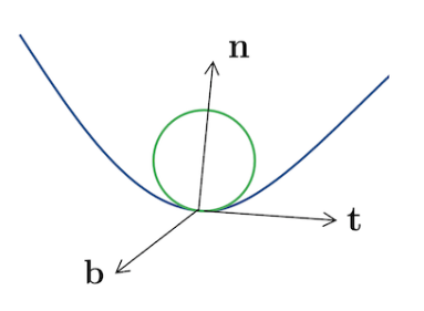
Note that the three vectors $\mathbf{t}$, $\mathbf{n}$ and $\mathbf{b}$ define an orthonormal basis for $\mathbb{R}^3$ at each point $s$ along the curve, which twists and turns along the curve.
Proposition. $d\mathbf{b}/ds$ is orthogonal to both $\mathbf{b}$ and $\mathbf{t}$ and therefore parallel to $\mathbf{n}$.
Proof.
Since $\vert \mathbf{b} \vert = 1$ for all $s$, we have $\mathbf{b} \cdot d\mathbf{b}/ds = 0$.
Since $\mathbf{t} \cdot \mathbf{b} = 0$, differentiating it and we have
\[0 = \kappa \mathbf{n} \cdot \mathbf{b} + \mathbf{t} \cdot {d \mathbf{b} \over ds}\]and $\mathbf{n} \cdot \mathbf{b} = 0$ so $\mathbf{t} \cdot d\mathbf{b}/ds = 0$
Definition. The torsion is the measure of how the binormal changes, defined by
\[{d\mathbf{b} \over ds} = -\tau \mathbf{n}\]
Proposition. [Frenet-Serret Equations]
\[{d\mathbf{t} \over ds} = \kappa \mathbf{n} \qquad {d\mathbf{b} \over ds} = -\tau \mathbf{n} \qquad {d\mathbf{n} \over ds} = \tau \mathbf{b} - \kappa \mathbf{t}\]Proof.
Since $\mathbf{b} \times \mathbf{t} = \mathbf{n}$, differentiating it and we have
\[{d\mathbf{n} \over ds} = {d\mathbf{b} \over ds} \times \mathbf{t} + \mathbf{b} \times {d\mathbf{t} \over ds} = -\tau (\mathbf{n} \times \mathbf{t}) + \kappa (\mathbf{b} \times \mathbf{n}) = \tau \mathbf{b} - \kappa \mathbf{t}\]
Surfaces
Definition. A parameterised surface $S$ is a vector function of the form $\mathbf{r}: \mathbb{R}^2 \to \mathbb{R}^3$.
We can also represent a surface by $z = f(x, y)$ or $F(x, y, z) = 0$ and convert them to parametric form by for example, having
\[\mathbf{r}(u, v) = u \mathbf{i} + v \mathbf{j} + f(u, v) \mathbf{k}\]Definition. The two curves $u = $ constant and $v = $ constant passing through $P$ on $S$ are called coordinate curves.
Definition. A normal vector $\mathbf{n}$ of $P$ on $S$ is the vector which points perpendicularly away from the surface. For the parameterised surface $\mathbf{r}(u, v) \in \mathbb{R}^3$, the normal direction is
\[\mathbf{n} = {\partial \mathbf{r} \over \partial u} \times {\partial \mathbf{r} \over \partial v}\]It is the normal vector of the tangent plane.
Definition. A parameterisation is regular if $\mathbf{n} \not= 0$ anywhere on the surface.
The sign of the normal vector determines what we mean by “outside” and “inside” the surface, and
Definition. A surface is orientable if there is a consistent choice of unit normal which varies smoothly over the surface.
Proposition. An infinitesimal vector displacement $d\mathbf{r}$ in the position of $P$ is given by
\[d\mathbf{r} = {\partial \mathbf{r} \over \partial u} du + {\partial \mathbf{r} \over \partial v} dv\]
Proposition. The area of the infinitesimal parallelogram whose sides are the coordinate curves is
\[dS = \left| {\partial \mathbf{r} \over \partial u} du \times {\partial \mathbf{r} \over \partial v} dv \right| = \left| {\partial \mathbf{r} \over \partial u} \times {\partial \mathbf{r} \over \partial v} \right| \,du \,dv = |\mathbf{n}| \,du \,dv\]
Definition. The infinitesimal vector area is defined to be
\[d\mathbf{S} = \mathbf{n} \,dS = \left( {\partial \mathbf{r} \over \partial u} \times {\partial \mathbf{r} \over \partial v} \right) {|\mathbf{n}| \over |\mathbf{n}|} \,du \,dv = \left( {\partial \mathbf{r} \over \partial u} \times {\partial \mathbf{r} \over \partial v} \right) \,du \,dv\]
Definition. A surface $S$ can have a boundary which is a piecewise smooth closed curve, denoted by $\partial S$.
For example, a sphere truncated by the $z = 0$ plane has boundary $x^2 + y^2 = R^2$ in the $z = 0$ plane.
Proposition. The boundary of a boundary has no boundary, i.e. $\partial^2 = 0$.
Definition. A surface is bounded if it can be contained within some solid sphere of fixed radius, otherwise it is unbounded.
Definition. A bounded surface with no boundary is closed.
Scalar and Vector Fields
We can also define a particular scalar or vector quantity continuously as a field throughout some region of space.
Definition. A scalar field is a scalar function of the form $\phi(\mathbf{x}): \mathbb{R}^3 \to \mathbb{R}$, which associates a scalar with each point in space.
Definition. The differential $d\phi$ is given by
\[d\phi = {\partial f \over \partial x_j} dx_j\]
For example, the pressure at each point in a fluid is a scalar field.
Definition. A vector field is a vector function of the form $\mathbf{F}(\mathbf{x}): \mathbb{R}^3 \to \mathbb{R}^3$, which associates a vector with each point in space.
For example, the electric field is a vector field.
Definition. The differential $d\mathbf{F}$ is given by
\[d\mathbf{F} = {\partial \mathbf{F} \over \partial x_j} dx_j\]
References
- David Tong Vector Calculus Lecture Notes, 2024 - Chapter 1.1, 2.2
- K.F. Riley Mathematical Methods for Physicists and Engineers, 1998 - Chapter 10.3, 10.5, 10.6